Neural Networks
Contents
Neural Networks
Intro
The shining star of learning algorithms are neural networks, and it’s likely that you’ve heard of them in some form before this chapter. Neural networks are extremely powerful in that they can do both classification and regression, and even learn their own features.
Neural networks are a culmination of the topics we’ve discussed in this book so far:
Perceptrons
Logistic Regression
Ensemble Learning
Stochastic Gradient Descent
Higher-dimensional feature vector lifting
Let’s go back a few chapters: all the way back to perceptrons. Remember that perceptrons were basically machines that came up with a linear decision boundary. Of course, there are inherent limitations to what a perceptron can do, particularly XOR:
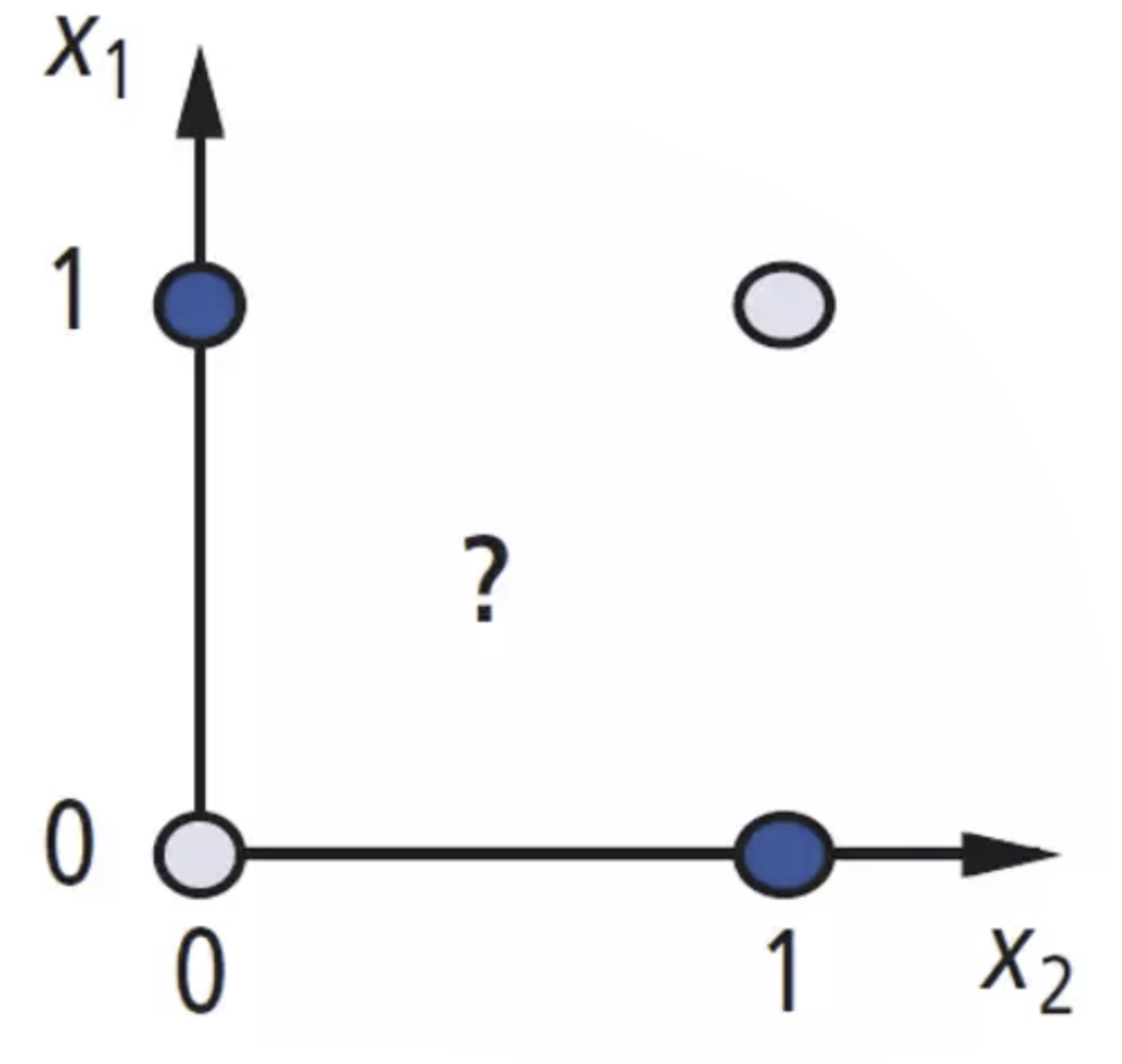
Here, we simply convert the XOR truth table to four points in 2-dimensional (binary) feature space. Blue points correspond to 1, while white points correspond to 0? Note that no matter how hard you try, you cannot find a linear separator that separates blue from white.
The fact that the perceptron showed such limitations on even “simple” problems like these drastically slowed research in the neural network field, for about a decade. Tough.
But there exist many simple solutions for this. One is adding a quadratic feature \(x_1x_2\)- effectively lifting our points to 3-dimensional feature space. Now, XOR is linearly separable.
But what about another way? Say we want to calculate \(X\) XOR \(Y\). We know that perceptrons output a linear combination of its inputs. What if we chained multiple perceptrons together like this, for inputs \(X\) and \(Y\). Can \(Z\) be the XOR of \(X\) and \(Y\)?

No. In all, all we have from chaining linear combos in this manner is just another linear combination. So equivalently, we just have another perceptron- will only work for linearly separable points.
We need to implement in between the initial perceptron outputs. Let us call the linear combo boxes neurons, although they may sometimes be referred to as units. If a neuron’s output is run through some nonlinear function before it goes to the next neuron as an input, then we may be able to simulate logic gates, and from there we might be able to build XOR.
There are many choices for this nonlinearity function. One that is often used is the logistic function. Remember the logistic function has range \([0,1]\), which is like an inherent normalization that ensures other neurons cannot be overemphasized. The function is also smooth: it has well-defined gradients and Hessians we can use for optimization.
Here’s a two-level perceptron with a logistic activation function that implements XOR:

Can an algorithm learn a function like this?
Training Neural Networks
We usually utilize stochastic or batch gradient descent to train neural networks. We need to pick a loss function \(L(z, y)\): usually, this is the squared norm: \(L(z,y) = ||z-y||^2\), and cost function \(J(h) = \frac{1}{n}\sum_{i=1}^{n}L(h(X_i), Y_i)\). Note that a single output for a data point is not a scalar but a vector. Therefore, outputs \(Y_i\) is a row of output matrix \(Y\). Sometimes there is just one output unit, but many neural net applications have more.
The goal is to find the optimal weights of the neural network that minimize \(J\): specifically, the optimal weight matrices \(V, W\) (there are more in NNs with more than one hidden layer, of course).
For neural networks, generally there are many local minima. The cost function for neural networks are generally not even close to convex. For that reason, it’s possible to end up at a bad minimum. In a later note, we’ll discuss some approaches for getting better minima out of neural nets.
So what’s the process of training?
Let’s start with a naïve approach. Suppose we start by setting all the weights to zero (\(W, V = 0\)), then apply gradient descent on the weights. Will this work?
Neural networks have a symmetry: there’s really no difference between one hidden unit and any other hidden unit. So if we start at a symmetric set of weights, the gradient descent algorithm won’t ever break this symmetry (unless optimal weights are symmetric, which is incredibly unlikely).
So to avoid this problem, to train neural networks we start with random weights.
Now we can apply gradient descent. Let \(w\) be a vector of all weights in \(V\) and \(W\). In batch gradient descent:
w = randomWeights()
while True:
	w = w - epsilon * gradient(J(w))
Note that in code, you should probably operate directly on \(V,W\) instead of concatenating everything for the sake of speed.
Additionally, it’s important to make sure our initial random weights aren’t too big: if a unit’s output gets too close to zero or one, it can get “stuck,” meaning that a modest change in the input values causes barely any change in the output value. Stuck units tend to stay stuck because in that operating range, the gradient \(s_0(·)\) of the logistic function is close to zero.
How do we compute \(\nabla_w J(w)\)? Naively, we calculate one derivative per weight, so for a network with multiple hidden layers, it takes time linear in the number of edges in the neural network to compute a derivative for one weight. For example, take the neural network below, with edges labeled:
Multiply that by the number of weights. So we get runtime \(O(\text{# edges}^2)\), and backpropagation takes \(O(\text{# edges})\). With complicated neural networks, this will get bad very quickly.
Computing Gradients for Arithmetic Expressions
Before we delve into the wonderful process of backpropagation, let us first view calculating the gradient for arithmetic expressions.
First, say we have the simple network below:
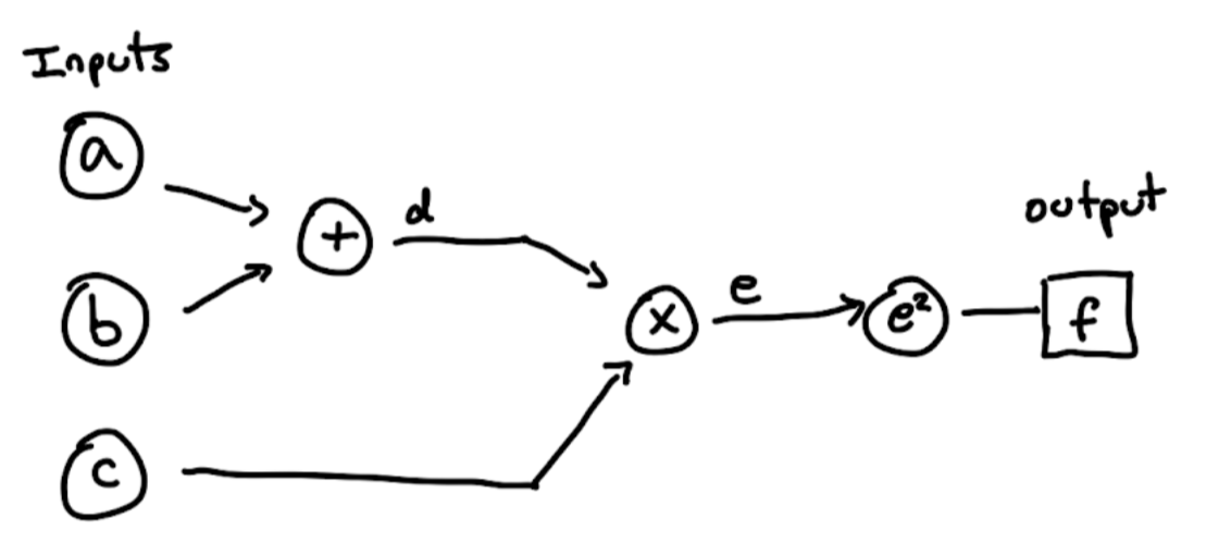
Notice we take in 3 scalar inputs \((a,b,c)\), perform a series of operations on them, and produce a scalar output \(f\).
In order to do gradient descent, we must compute the gradient of \(f\) with respect to our inputs \(a,b,c\): \(\nabla f = \begin{bmatrix} \frac{\partial f}{\partial a} \\ \frac{\partial f}{\partial b} \\ \frac{\partial f}{\partial c} \end{bmatrix}\).
In order to find such partial derivatives, we must do things one layer at a time and apply the chain rule. Let’s start at \(\frac{\partial f}{\partial a}\), and use \(d\) as an intermediary:
We can immediately calculate one of these terms: we know that \(\frac{\partial d}{\partial a} = \frac{\partial}{\partial a}(a+b) = 1\). Additionally, we’ll note that \(\frac{\partial d}{\partial b} = 1\) as we’ll use this later. So what’s left now is to calculate a partial derivative that is one layer closer: \(\frac{\partial f}{\partial a} = \frac{\partial f}{\partial d} * 1\). We can’t really calculate this at the moment, so we save it as a subtask for now, and we’ll do some other calculations to hopefully be able to calculate it later. Note this is very characteristic of dynamic programming: in fact, that is exactly what this process is!
So now, we move on to \(\frac{\partial f}{\partial b} = \frac{\partial f}{\partial d} \cdot \frac{\partial d}{\partial b} = \frac{\partial f}{\partial d}\). Still no good. On to the next one.
Finally, we calculate \(\frac{\partial f}{\partial c}\). Viewing downstream, we see that the \(e\) node, so we’ll use \(e\) as an intermediary this time:
Again, we can compute \(\frac{\partial e}{\partial c} = \frac{\partial}{\partial c}cd = d\). We’ll also note that \(\frac{\partial}{\partial d}cd = c\).
So in all, we have established our base equations, starting from the input:
So now all we’re left with is calculating \(\frac{\partial f}{\partial d}\) and \(\frac{\partial f}{\partial e}\). The way to do this is just to move downstream: instead of our “starting nodes” being a,b,c, we just treat our starting nodes as d,e and derive some more equations from there!
So we repeat the same exact process: find the intermediary node and use the chain rule. Doing this gives us equations
Hurray! We finally have a partial derivative for one of the weights. We can now utilize the backpropagation process and substitute everything from output layer to input layer, which give us our final gradients:
So we have successfully used dynamic programming to solve the gradients at each layer. So now we have our gradient \(\nabla f\) with respect to our input weights!
That was quite a mouthful, so let’s recap. Each value that we calculate \(z\) gives a partial derivative of the form \(\frac{\partial f}{\partial z} = \frac{\partial f}{\partial n} \cdot \frac{\partial n}{\partial z}\), where \(f\) is the output of the network and \(n\) is a node one layer downstream of \(z\): in other words, \(z\) is an input to \(n\). We have a forward pass and a backwards pass. In the forwards pass, where we go left to right, we calculate \(\frac{\partial n}{\partial z}\): the intermediary partial derivatives are calculated. In the backwards pass, where we go in the reverse direction from right to left, we compute \(\frac{\partial f}{\partial n}\). Information from the right end of the network is literally propagated backwards to the left (back-propagation).
Note
In practice, backpropagation usually refers to the entire process: both the forward and backwards pass. Don’t get confused.
Extending to Single-Output-Multiple Input
Let’s extend this process to when a node’s output acts as multiple inputs in the next layer. Let’s take a look at an example network that does this:
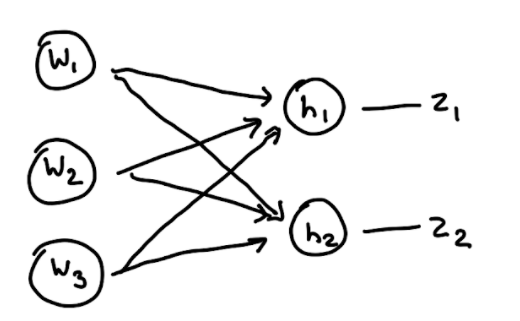
Note that each input \(w_1, w_2, w_3\) now serves as inputs to MULTIPLE downstream nodes. Let’s assume \(h_1 = X_{11}w_1 + X_{22}w_2 + w_3\), and \(h_2 = X_{21}w_1 + X_{22 }w_2 + w_3\). The outputs \(z = (z_1, z_2)\) are input into a loss function \(L(z,y) = ||z-y||^2\).
How can we do backpropagation here? Well, the goal stays the same: we want to calculate the gradient of \(L\) as \(\nabla L = \begin{bmatrix} \frac{\partial L}{\partial w_1} \\ \frac{\partial L}{\partial w_2} \\ \frac{\partial L}{\partial w_3} \end{bmatrix}\). However, note that each of the input weights influences the loss between hidden nodes \(z_1\) AND \(z_2\). So now we have a sort of multivariate system of differential equations.
We know that
I’ll leave it to you to follow the logic and write out the corresponding expressions for \(\frac{\partial L}{\partial w_2}\) and \(\frac{\partial L}{\partial w_3}\). Note that \(w_3\) is our bias term, so we know that \(\frac{\partial z_1}{\partial w_3} = \frac{\partial z_1}{\partial w_3} = 1\).
Following the downstream forward pass process, we then find \(\frac{\partial L}{\partial z_1} = 2(z_1 - y_1)\), and \(\frac{\partial L}{\partial z_2} = 2(z_2 - y_2)\). Now during the backwards pass, we do the same backpropagation: except now these values go to three places instead of just one like before.
Remember that \(\frac{\partial}{\partial \tau}L(z_1(\tau), z_2(\tau)) = \nabla_z L \cdot \frac{\partial}{\partial \tau} z\). We need this equation for backpropagation.
So the fact that we are utilizing dynamic programming in these passes allows us to reduce runtime from \(O(\text{# edges}^2)\) to \(O(\text{# edges})\): a huge improvement.
The Backpropagation Algorithm
Let’s formalize this algorithm as it’s used in neural networks. The backpropagation algorithm is a DP algorithm to compute the gradients for neural network gradient descent, in runtime linear to the number of weights (edges). We represent \(V_i^T\) as row \(i\) of a weight matrix \(V\).
Remember that the output value of the \(i\)-th node in the hidden layer is denoted as \(h_i = s(V_i \cdot x)\), where \(s\) is a logistic activation function. This means that the gradient for a hidden layer node \(\nabla_{V_i}h_i = s'(V_i \cdot x)x\) by the chain rule. We can further simplify this down to \(\nabla_{V_i}h_i = h_i(1-h_i)x\).
We also need gradients for the output layer node with respect to our weights. Let’s assume we use a logistic activation function for outputs too (but this doesn’t have to be the case). Let \(z_j = s(W_j \cdot h)\) be the output of the \(j\)-th output node. This means \(\nabla_{W_j}z_j = s'(W_j \cdot h)h = z_j(1-z_j)h\).
Finally, we also need to calculate the gradient of the output layer with respect to the hidden layer weights- completing the connection. We calculate \(\nabla_h z_j = z_j(1-z_j)W_j\).
Let us now reformulate our neural network, where our inputs are the weight matrices \(W,V\) instead of individual weights:
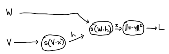
Now for our forward pass: we are calculating the gradients with respect to \(W,V\): we want \(\nabla_{V} L\) and \(\nabla_{W} L\). Specifically, we can calculate \(\nabla_{W_j}L = \frac{\partial L}{\partial z_j} z_j(1-z_j)h\) as well as \(\nabla_{V_i}L = \frac{\partial L}{\partial h_i} h_i(1-h_i)x\).
Now in the backwards pass, we move backwards to plug in \(\nabla_z L = 2(z-y)\), and \(\nabla_h L = \sum_{j}z_j(1-z_j)\nabla_z L W_j\), which we plug in as \(\nabla_h L = \sum_{j}z_j(1-z_j) \cdot 2(z-y) W_j\).
So we’ve found the gradient of the neural network using backpropagation for a general neural network!